
Capillary Pressure data integration helps defining carbonates reservoir compartmentalization
- Francisco Caycedo

- Nov 27, 2020
- 5 min read

This post is about an interesting example of how the capillary pressure data integrated with other information helped to understand the compartmentalization of a carbonate field that was under water injection.
One of the potential problems affecting the efficiency of water injection techniques is the areal variation of the rock quality. In this case study, a permeability barrier was preventing that one part of the field benefits from the waterflooding influence. No faulting or any other structural feature was observed in the seismic.
Quick Field Description
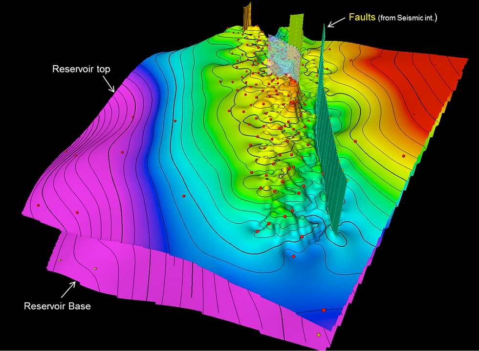
The structure of this Mesozoic carbonates reservoir can be described as an anticline limited by a system of faults in one flank. In the picture to the right are presented the top and base surfaces and the main faults interpreted in the seismic.
Several cores were cut in different wells of the field and capillary pressure, porosity and permeability were measured among other properties.

As a reference, in the picture to the left is presented the petrophysical analysis of one of the wells. Track 1 shows GR, track 2 water saturation and irreducible water saturation estimation (blue), tracks 3 and 4 porosity (including core data), track 5 mineralogy, track 6 rock typing and track 7 permeability functions (including core data).
The dashed blue line crossing all the tracks represents the computed Free Water Level (FWL).
Free Water Level (FWL) Calculation
FWL was calculated in several wells using saturation height modeling based on capillary pressure curves and Leverett J-Function (1). The general workflow is described below and some other details related to the process are presented at the end of this post (Appendix A).

Capillary pressure curves were validated, corrected (conformance correction), and converted to the same system (air-mercury) and units.
Rock typing analysis was performed to classify capillary pressure (Pc) curves in groups according to porosity, permeability and pore throat radius. In this specific case, porosity ranges segregated very well Pc curves, but this varies from reservoir to reservoir.
Leverett J-Functions were computed for each Pc curve: J = 0.2166 * [Pc/(σ * Cos(Θ))] * (K/PHI)^0.5
Wetting phase Saturation vs. J-Function was plotted (Log-Log) and regressions performed considering the points within each rock type to obtain equations of the form: J = a * Sw ^ b. These equations were rearranged to Sw= ( J / a ) ^ (1/b).
In the previous step sometimes wetting phase Saturation needs to be normalized by Swirr in order to get a better fit. In this case the resulting equations in the regression have the following form: Swn= ( J / a ) ^ (1/b) and a de-normalization function is required later to compute Sw. The de-normalization function is a equation that correlates Swirr with other parameter like PHI, log(PHI), log(K) or log(Ri).
An example of de-normalization function based on log(PHI) is
Swirr= -1.13892 * Log(PHI) + 1.24808
Sw = Swirr + Swn * (1 - Swirr)
A Saturation Height model was defined by Combining the equations previously described with the general Capillary Pressure equation for each rock type: Pc = (rhoW - rhoH) * h / 703.07, where h represents the FWL
Eq.1 Sw= ( J / a ) ^ (1/b)
Eq.2 J = 0.2166 * [Pc/(σ * Cos(Θ))] * (K/PHI)^0.5
Eq.3 Pc = (rhoW - rhoH) * FWL / 703.07
Sw = {(0.2166 * [((rhoW-rhoH) * FWL / 703.07) / (σ*Cos(Θ))] *(K/PHI)^0.5)/a}^(1/b) Eq.4
This equation is defined by each rock type by changing the a and b variables (calculated in the Sw vs. J-function regression).
Pc = capillary pressure, psi
σ = system interfacial tension, dynes/cm
Θ = contact angle, degrees
K = permeability, mD
PHI = porosity, v/v
h = free water level (FWL), meters
rhoW = water density, Kg/m3
rhoH = hydrocarbon density, Kg/m3
Sw = wetting phase saturation, fraction
Swn = wetting phase saturation normalized by Swirr, fraction
Swirr = irreducible wetting phase saturation, fraction
Ri = pore throat radius, microns
Finally, because continuous porosity, permeability and water saturation curves were previously calculated during the petrophysical analysis, FWL was iterated until getting the best match between the SW computed from well logs and the one computed in the Saturation Height model (Eq.4)
Free Water Level (FWL) Analysis and Results
Using the workflow explained in the previous section, the FWL was calculated in 13 wells. The most interesting observation was that two different FWL were estimated in the group of wells. For a group of 7 wells the FWL required to have a good match between the water saturation calculated from the well logs and the calculated from the saturation height modeling was -2,820 m. For the other group of 6 wells the required FWL was -2,870 m.
In the picture below is presented an example of the FWL estimation in one of the wells. At the left side is shown that a FWL=-2,820 m produces a poor match. At the right side is shown that a FWL=-2,870 m produces a good match.

In the picture below is presented another example where the best match is obtained by using a FWL=-2,820 m.


When the 2 groups of wells were displayed in a map, all the 6 wells with deeper FWL were located to the north of the group of 7 wells with shallower FWL (see picture to the left).
The presence of 2 different FWL suggested compartmentalization in the reservoir and helped to better understand the dynamic behaviour and the effect of the waterflooding process in some wells.

The picture to the right shows a Phi*H map filtered by porosity higher than 6%, suggesting that the barrier is probably caused by a change in rock quality, given that not structural features were observed in the seismic.
As a final comment, a geological model was built integrating the all the data presented in this post (including rock typing and water saturation from the saturation height model), followed by numeric simulation with excellent history match.

Appendix A
Capillary Pressure Conformance Correction
Within the corrections applied to the mercury injection capillary pressure data is the conformance correction. It refers to the amount of mercury that conforms to the exterior shape of the plug and the contact between the plug and its enclosing holder. This "apparent" intrusion of mercury into the sample must be discounted or corrected and it’s critical for some calculations like permeability estimation from MICP data.
Picture below shows an example of the graphs used in the correction of one of the samples analyzed in this case study.

Rock Typing for Saturation Height Modeling
As mentioned in the general workflow description, Rock-typing analysis was performed to classify capillary pressure (Pc) curves in families or groups according to porosity, permeability and pore throat radius. Then a saturation height equation was derived for each rock type. This is a very important step when using Levertt J-Function methodology.
In the picture below are shown examples of capillary pressure data from 3 different reservoirs. In the example to the left, permeability ranges allowed to group the Pc curves with similar behaviour. In the example presented in the middle, porosity ranges effectively group Pc curves with similar characteristics. Finally, in the example to the right the Pc curves are grouped by pore throat radius (R45 port).

There are several options when grouping Pc curves by pore throat radius. One of the most common procedures consists in finding the most representative Winland or Pittman equation (2). This could be done by:
Computing the pore throat aperture (R) at Pc values corresponding to different saturations (ports), using the Young-Laplace equation: R = (2σ * Cos(Θ))/ Pc
Computing the different Winland and Pittman apparent radius (R10, 15, 20, 25,… 75)
Plotting Critical Pore Aperture (Young-Laplace equation) vs. Winland/Pittman Apparent Radius for each port (saturation) and finding the combination with better correlation.
Plotting Porosity vs Permeability data (colouring points by Critical Pore Aperture), displaying selected Winland/Pittman correlation overlay lines, and comparing the results. Points within a specific group of critical pore aperture should be in agreement with the corresponding Winland/Pittman lines.
Apex plots (Non-wetting phase saturation vs. Saturation/Capillary pressure) and Pore Throat Size Distribution plots are also helpful diagnostic tools.

References
Leverett, M.C.: “Capillary behaviour in porous solids” Petroleum Transactions of AIME 142 (1941)
Pittman, E.D.: "Relationship of Porosity and Permeability to Various Parameters Derived from Mercury Injection-Capillary Pressure Curves for Sandstone," AAPG Bull., vol. 76, No. 2 (February 1992)


Comments